Optimization Methods: GD, Mini-batch GD, Momentum, RMSProp, Adam
Optimization Methods
import numpy as np
import matplotlib.pyplot as plt
import scipy.io
import math
import sklearn
import sklearn.datasets

from opt_utils import load_params_and_grads, initialize_parameters, forward_propagation, backward_propagation
from opt_utils import compute_cost, predict, predict_dec, plot_decision_boundary, load_dataset
from testCases import *

%matplotlib inline
plt.rcParams['figure.figsize'] = (7.0, 4.0) # set default size of plots
plt.rcParams['image.interpolation'] = 'nearest'
plt.rcParams['image.cmap'] = 'gray'
1- Gradient Descent (GD)
A simple optimization method in machine learning is gradient descent (GD). When you take gradient steps with respect to all mm examples on each step, it is also called Batch Gradient Descent.
def update_parameters_with_gd(parameters, grads, learning_rate):
    """
    Update parameters using one step of gradient descent

    Arguments:
    parameters -- python dictionary containing your parameters to be updated:
                    parameters['W' + str(l)] = Wl
                    parameters['b' + str(l)] = bl
    grads -- python dictionary containing your gradients to update each parameters:
                    grads['dW' + str(l)] = dWl
                    grads['db' + str(l)] = dbl
    learning_rate -- the learning rate, scalar.

    Returns:
    parameters -- python dictionary containing your updated parameters
    """

    L = len(parameters) // 2 # number of layers in the neural networks

    # Update rule for each parameter
    for l in range(L):
        parameters["W" + str(l+1)] = parameters['W' + str(l+1)] - learning_rate*grads['dW' + str(l+1)]
        parameters["b" + str(l+1)] = parameters["b" + str(l+1)] - learning_rate*grads['db' + str(l+1)]

    return parameters
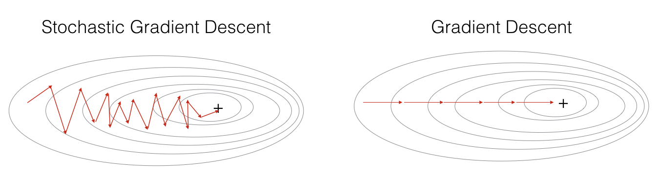
A variant of this is Stochastic Gradient Descent (SGD), which is equivalent to mini-batch gradient descent where each mini-batch has just 1 example. The update rule that we have just implemented does not change. What changes is that you would be computing gradients on just one training example at a time, rather than on the whole training set. The code examples below illustrate the difference between stochastic gradient descent and (batch) gradient descent.
- (Batch) Gradient Descent:
X = data_input
Y = labels
parameters = initialize_parameters(layers_dims)
for i in range(0, num_iterations):
    # Forward propagation
    a, caches = forward_propagation(X, parameters)
    # Compute cost.
    cost = compute_cost(a, Y)
    # Backward propagation.
    grads = backward_propagation(a, caches, parameters)
    # Update parameters.
    parameters = update_parameters(parameters, grads)
- Stochastic Gradient Descent:
X = data_input
Y = labels
parameters = initialize_parameters(layers_dims)
for i in range(0, num_iterations):
    for j in range(0, m):
        # Forward propagation
        a, caches = forward_propagation(X[:,j], parameters)
        # Compute cost
        cost = compute_cost(a, Y[:,j])
        # Backward propagation
        grads = backward_propagation(a, caches, parameters)
        # Update parameters.
        parameters = update_parameters(parameters, grads)
In Stochastic Gradient Descent, you use only 1 training example before updating the gradients. When the training set is large, SGD can be faster. But the parameters will “oscillate” toward the minimum rather than converge smoothly. Here is an illustration of this:
What to remember:
- The difference between gradient descent, mini-batch gradient descent and stochastic gradient descent is the number of examples you use to perform one update step.
- You have to tune a learning rate hyperparameter α .
- With a well-turned mini-batch size, usually it outperforms either gradient descent or stochastic gradient descent (particularly when the training set is large).
2- Mini-batch Gradient Descent
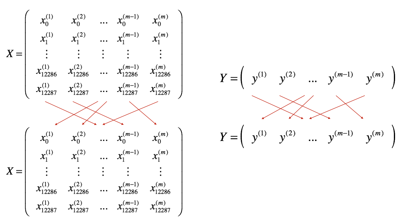
Shuffle: Create a shuffled version of the training set (X, Y) as shown below. Each column of X and Y represents a training example. Note that the random shuffling is done synchronously between X and Y. Such that after the shuffling the i’th column of X is the example corresponding to the i’th label in Y. The shuffling step ensures that examples will be split randomly into different mini-batches.
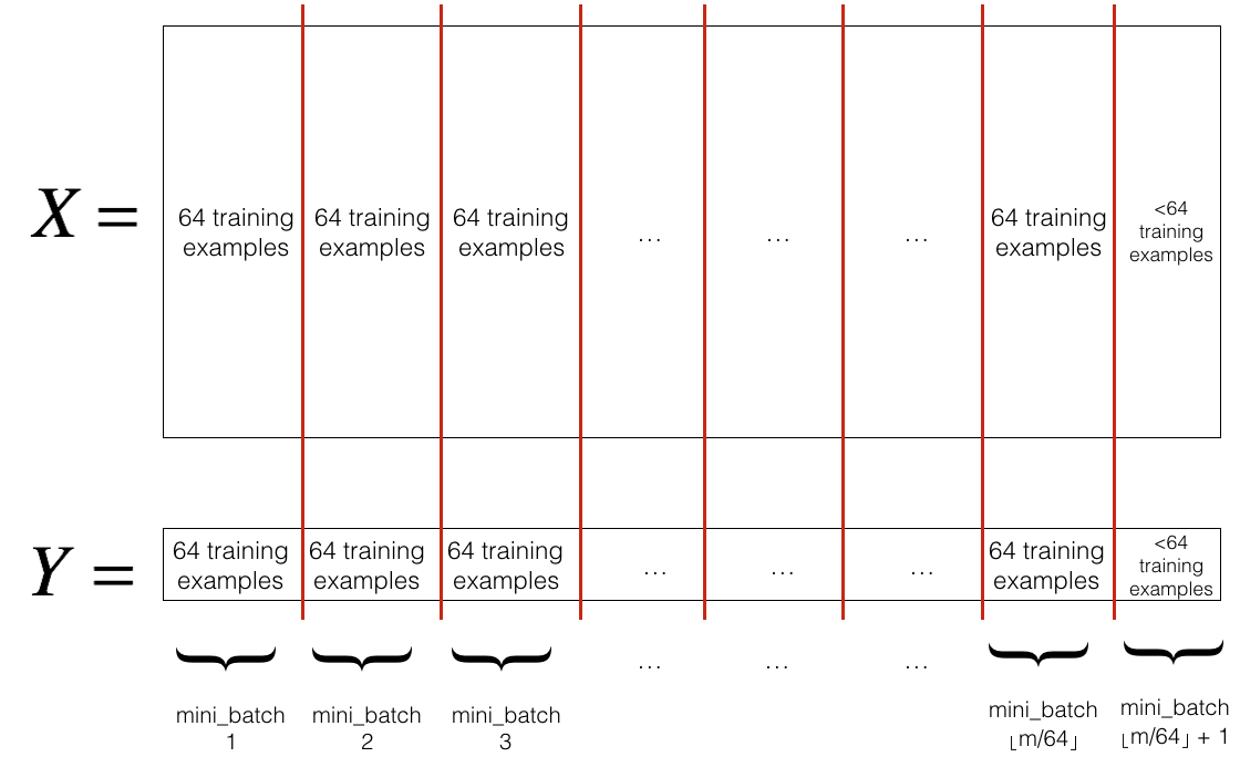
Partition: Partition the shuffled (X, Y) into mini-batches of size mini_batch_size (here 64). Note that the number of training examples is not always divisible by mini_batch_size. The last mini batch might be smaller, but you don’t need to worry about this. When the final mini-batch is smaller than the full mini_batch_size, it will look like this:
def random_mini_batches(X, Y, mini_batch_size = 64, seed = 0):
    """
    Creates a list of random minibatches from (X, Y)

    Arguments:
    X -- input data, of shape (input size, number of examples)
    Y -- true "label" vector (1 for blue dot / 0 for red dot), of shape (1, number of examples)
    mini_batch_size -- size of the mini-batches, integer

    Returns:
    mini_batches -- list of synchronous (mini_batch_X, mini_batch_Y)
    """

    np.random.seed(seed)            # To make your "random" minibatches the same as ours
    m = X.shape[1]                  # number of training examples
    mini_batches = []

    # Step 1: Shuffle (X, Y)
    permutation = list(np.random.permutation(m))
    shuffled_X = X[:, permutation]
    shuffled_Y = Y[:, permutation].reshape((1,m))

    # Step 2: Partition (shuffled_X, shuffled_Y). Minus the end case.
    num_complete_minibatches = math.floor(m/mini_batch_size) # number of mini batches of size mini_batch_size in your partitionning
    for k in range(0, num_complete_minibatches):
        mini_batch_X = shuffled_X[:, k*mini_batch_size : (k+1)*mini_batch_size]
        mini_batch_Y = shuffled_Y[:, k*mini_batch_size : (k+1)*mini_batch_size]
        mini_batch = (mini_batch_X, mini_batch_Y)
        mini_batches.append(mini_batch)

    # Handling the end case (last mini-batch < mini_batch_size)
    if m % mini_batch_size != 0:
        mini_batch_X = shuffled_X[:, (k+1)*mini_batch_size : m]
        mini_batch_Y = shuffled_Y[:, (k+1)*mini_batch_size : m]
        mini_batch = (mini_batch_X, mini_batch_Y)
        mini_batches.append(mini_batch)

    return mini_batches
What to remember:
- Shuffling and Partitioning are the two steps required to build mini-batches
- Powers of two are often chosen to be the mini-batch size, e.g., 16, 32, 64, 128.
3- Momentum
Because mini-batch gradient descent makes a parameter update after seeing just a subset of examples, the direction of the update has some variance, and so the path taken by mini-batch gradient descent will “oscillate” toward convergence. Using momentum can reduce these oscillations.
Momentum takes into account the past gradients to smooth out the update. We will store the ‘direction’ of the previous gradients in the variable vv . Formally, this will be the exponentially weighted average of the gradient on previous steps. You can also think of vv as the “velocity” of a ball rolling downhill, building up speed (and momentum) according to the direction of the gradient/slope of the hill.

def initialize_velocity(parameters):
    """
    Initializes the velocity as a python dictionary with:
                - keys: "dW1", "db1", ..., "dWL", "dbL"
                - values: numpy arrays of zeros of the same shape as the corresponding gradients/parameters.
    Arguments:
    parameters -- python dictionary containing your parameters.
                    parameters['W' + str(l)] = Wl
                    parameters['b' + str(l)] = bl

    Returns:
    v -- python dictionary containing the current velocity.
                    v['dW' + str(l)] = velocity of dWl
                    v['db' + str(l)] = velocity of dbl
    """

    L = len(parameters) // 2 # number of layers in the neural networks
    v = {}

    # Initialize velocity
    for l in range(L):
        v["dW" + str(l+1)] = np.zeros((parameters["W" + str(l+1)].shape[0],parameters["W" + str(l+1)].shape[1]))
        v["db" + str(l+1)] = np.zeros((parameters["b" + str(l+1)].shape[0],parameters["b" + str(l+1)].shape[1]))

    return v
Now we will implement updating parameters with momentum.

def update_parameters_with_momentum(parameters, grads, v, beta, learning_rate):
    """
    Update parameters using Momentum

    Arguments:
    parameters -- python dictionary containing your parameters:
                    parameters['W' + str(l)] = Wl
                    parameters['b' + str(l)] = bl
    grads -- python dictionary containing your gradients for each parameters:
                    grads['dW' + str(l)] = dWl
                    grads['db' + str(l)] = dbl
    v -- python dictionary containing the current velocity:
                    v['dW' + str(l)] = ...
                    v['db' + str(l)] = ...
    beta -- the momentum hyperparameter, scalar
    learning_rate -- the learning rate, scalar

    Returns:
    parameters -- python dictionary containing your updated parameters
    v -- python dictionary containing your updated velocities
    """

    L = len(parameters) // 2 # number of layers in the neural networks

    # Momentum update for each parameter
    for l in range(L):

        # compute velocities
        v["dW" + str(l+1)] = beta*v["dW" + str(l+1)]+(1-beta)*grads['dW' + str(l+1)]
        v["db" + str(l+1)] = beta*v["db" + str(l+1)]+(1-beta)*grads['db' + str(l+1)]
        # update parameters
        parameters["W" + str(l+1)] = parameters["W" + str(l+1)] - learning_rate*v["dW" + str(l+1)]
        parameters["b" + str(l+1)] = parameters["b" + str(l+1)] - learning_rate*v["db" + str(l+1)]

    return parameters, v
Note that:
-
The velocity is initialized with zeros. So the algorithm will take a few iterations to “build up” velocity and start to take bigger steps. If β=0 , then this just becomes standard gradient descent without momentum. How do you choose β ?
- The larger the momentum β is, the smoother the update because the more we take the past gradients into account. But if β is too big, it could also smooth out the updates too much.
- Common values for β range from 0.8 to 0.999. If you don’t feel inclined to tune this, β=0.9 is often a reasonable default.
- Tuning the optimal β for your model might need trying several values to see what works best in term of reducing the value of the cost function J.
What to remember:
- Momentum takes past gradients into account to smooth out the steps of gradient descent. It can be applied with batch gradient descent, mini-batch gradient descent or stochastic gradient descent.
- You have to tune a momentum hyperparameter β and a learning rate α .
4 - Adam
Adam is one of the most effective optimization algorithms for training neural networks. It combines ideas from RMSProp and Momentum.
How does Adam work?
- It calculates an exponentially weighted average of past gradients, and stores it in variables v (before bias correction) and v_corrected (with bias correction).
- It calculates an exponentially weighted average of the squares of the past gradients, and stores it in variables s (before bias correction) and s_cprrected (with bias correction).
- It updates parameters in a direction based on combining information from “1” and “2”.
- The update rule is, for l=1,…,L :
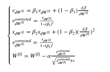
where:
- t counts the number of steps taken of Adam
- L is the number of layers
- β1 and β2 are hyperparameters that control the two exponentially weighted averages.
- α is the learning rate
- ε is a very small number to avoid dividing by zero
def initialize_adam(parameters) :
    """
    Initializes v and s as two python dictionaries with:
                - keys: "dW1", "db1", ..., "dWL", "dbL"
                - values: numpy arrays of zeros of the same shape as the corresponding gradients/parameters.

    Arguments:
    parameters -- python dictionary containing your parameters.
                    parameters["W" + str(l)] = Wl
                    parameters["b" + str(l)] = bl

    Returns:
    v -- python dictionary that will contain the exponentially weighted average of the gradient.
                    v["dW" + str(l)] = ...
                    v["db" + str(l)] = ...
    s -- python dictionary that will contain the exponentially weighted average of the squared gradient.
                    s["dW" + str(l)] = ...
                    s["db" + str(l)] = ...

    """

    L = len(parameters) // 2 # number of layers in the neural networks
    v = {}
    s = {}

    # Initialize v, s. Input: "parameters". Outputs: "v, s".
    for l in range(L):
        v["dW" + str(l+1)] = np.zeros((parameters["W" + str(l+1)].shape[0],parameters["W" + str(l+1)].shape[1]))
        v["db" + str(l+1)] = np.zeros((parameters["b" + str(l+1)].shape[0],parameters["b" + str(l+1)].shape[1]))
        s["dW" + str(l+1)] = np.zeros((parameters["W" + str(l+1)].shape[0],parameters["W" + str(l+1)].shape[1]))
        s["db" + str(l+1)] = np.zeros((parameters["b" + str(l+1)].shape[0],parameters["b" + str(l+1)].shape[1]))

    return v, s
def update_parameters_with_adam(parameters, grads, v, s, t, learning_rate = 0.01,
                                beta1 = 0.9, beta2 = 0.999,  epsilon = 1e-8):
    """
    Update parameters using Adam

    Arguments:
    parameters -- python dictionary containing your parameters:
                    parameters['W' + str(l)] = Wl
                    parameters['b' + str(l)] = bl
    grads -- python dictionary containing your gradients for each parameters:
                    grads['dW' + str(l)] = dWl
                    grads['db' + str(l)] = dbl
    v -- Adam variable, moving average of the first gradient, python dictionary
    s -- Adam variable, moving average of the squared gradient, python dictionary
    learning_rate -- the learning rate, scalar.
    beta1 -- Exponential decay hyperparameter for the first moment estimates
    beta2 -- Exponential decay hyperparameter for the second moment estimates
    epsilon -- hyperparameter preventing division by zero in Adam updates

    Returns:
    parameters -- python dictionary containing your updated parameters
    v -- Adam variable, moving average of the first gradient, python dictionary
    s -- Adam variable, moving average of the squared gradient, python dictionary
    """

    L = len(parameters) // 2                 # number of layers in the neural networks
    v_corrected = {}                         # Initializing first moment estimate, python dictionary
    s_corrected = {}                         # Initializing second moment estimate, python dictionary

    # Perform Adam update on all parameters
    for l in range(L):
        # Moving average of the gradients. Inputs: "v, grads, beta1". Output: "v".
        v["dW" + str(l+1)] = (beta1*v["dW" + str(l+1)])+((1-beta1)*grads['dW' + str(l+1)])
        v["db" + str(l+1)] = (beta1*v["db" + str(l+1)])+((1-beta1)*grads['db' + str(l+1)])

        # Compute bias-corrected first moment estimate. Inputs: "v, beta1, t". Output: "v_corrected".
        v_corrected["dW" + str(l+1)] = v["dW" + str(l+1)]/(1-(beta1**t))
        v_corrected["db" + str(l+1)] = v["db" + str(l+1)]/(1-(beta1**t))

        # Moving average of the squared gradients. Inputs: "s, grads, beta2". Output: "s".
        #(np.multiply(parameters['W' + str(l+1)],parameters['W' + str(l+1)]))
        s["dW" + str(l+1)] = (beta2*s["dW" + str(l+1)])+((1-beta2)*((grads['dW' + str(l+1)])**2))
        s["db" + str(l+1)] = (beta2*s["db" + str(l+1)])+((1-beta2)*((grads['db' + str(l+1)])**2))


        # Compute bias-corrected second raw moment estimate. Inputs: "s, beta2, t". Output: "s_corrected".
        s_corrected["dW" + str(l+1)] = s["dW" + str(l+1)]/(1-(beta2**t))
        s_corrected["db" + str(l+1)] = s["db" + str(l+1)]/(1-(beta2**t))


        # Update parameters. Inputs: "parameters, learning_rate, v_corrected, s_corrected, epsilon". Output: "parameters".
        parameters["W" + str(l+1)] = parameters["W" + str(l+1)] - learning_rate*(v_corrected["dW" + str(l+1)]/(np.sqrt(s_corrected["dW" + str(l+1)])+epsilon))
        parameters["b" + str(l+1)] = parameters["b" + str(l+1)] - learning_rate*(v_corrected["db" + str(l+1)]/(np.sqrt(s_corrected["db" + str(l+1)])+epsilon))

    return parameters, v, s
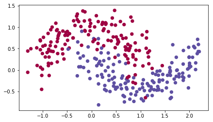
5 - Model with Optimization Algorithms
Lets use the following “moons” dataset to test the different optimization methods. (The dataset is named “moons” because the data from each of the two classes looks a bit like a crescent-shaped moon.)
train_X, train_Y = load_dataset()
We have already implemented a 3-layer neural network. You will train it with:
- Mini-batch Gradient Descent: it will call your function:
update_parameters_with_gd()
- Mini-batch Momentum: it will call your functions:
initialize_velocity()andupdate_parameters_with_momentum()
- Mini-batch Adam: it will call your functions:
initialize_adam()andupdate_parameters_with_adam()
def model(X, Y, layers_dims, optimizer, learning_rate = 0.0007, mini_batch_size = 64, beta = 0.9,
          beta1 = 0.9, beta2 = 0.999,  epsilon = 1e-8, num_epochs = 10000, print_cost = True):
    """
    3-layer neural network model which can be run in different optimizer modes.

    Arguments:
    X -- input data, of shape (2, number of examples)
    Y -- true "label" vector (1 for blue dot / 0 for red dot), of shape (1, number of examples)
    layers_dims -- python list, containing the size of each layer
    learning_rate -- the learning rate, scalar.
    mini_batch_size -- the size of a mini batch
    beta -- Momentum hyperparameter
    beta1 -- Exponential decay hyperparameter for the past gradients estimates
    beta2 -- Exponential decay hyperparameter for the past squared gradients estimates
    epsilon -- hyperparameter preventing division by zero in Adam updates
    num_epochs -- number of epochs
    print_cost -- True to print the cost every 1000 epochs

    Returns:
    parameters -- python dictionary containing your updated parameters
    """

    L = len(layers_dims)             # number of layers in the neural networks
    costs = []                       # to keep track of the cost
    t = 0                            # initializing the counter required for Adam update
    seed = 10                        # For grading purposes, so that your "random" minibatches are the same as ours

    # Initialize parameters
    parameters = initialize_parameters(layers_dims)

    # Initialize the optimizer
    if optimizer == "gd":
        pass # no initialization required for gradient descent
    elif optimizer == "momentum":
        v = initialize_velocity(parameters)
    elif optimizer == "adam":
        v, s = initialize_adam(parameters)

    # Optimization loop
    for i in range(num_epochs):

        # Define the random minibatches. We increment the seed to reshuffle differently the dataset after each epoch
        seed = seed + 1
        minibatches = random_mini_batches(X, Y, mini_batch_size, seed)

        for minibatch in minibatches:

            # Select a minibatch
            (minibatch_X, minibatch_Y) = minibatch

            # Forward propagation
            a3, caches = forward_propagation(minibatch_X, parameters)

            # Compute cost
            cost = compute_cost(a3, minibatch_Y)

            # Backward propagation
            grads = backward_propagation(minibatch_X, minibatch_Y, caches)

            # Update parameters
            if optimizer == "gd":
                parameters = update_parameters_with_gd(parameters, grads, learning_rate)
            elif optimizer == "momentum":
                parameters, v = update_parameters_with_momentum(parameters, grads, v, beta, learning_rate)
            elif optimizer == "adam":
                t = t + 1 # Adam counter
                parameters, v, s = update_parameters_with_adam(parameters, grads, v, s,
                                                               t, learning_rate, beta1, beta2,  epsilon)

        # Print the cost every 1000 epoch
        if print_cost and i % 1000 == 0:
            print ("Cost after epoch %i: %f" %(i, cost))
        if print_cost and i % 100 == 0:
            costs.append(cost)

    # plot the cost
    plt.plot(costs)
    plt.ylabel('cost')
    plt.xlabel('epochs (per 100)')
    plt.title("Learning rate = " + str(learning_rate))
    plt.show()

    return parameters
5.1 Mini-batch Gradient descent
Lets run the following code to see how the model does with mini-batch gradient descent.
# train 3-layer model
layers_dims = [train_X.shape[0], 5, 2, 1]
parameters = model(train_X, train_Y, layers_dims, optimizer = "gd")

# Predict
predictions = predict(train_X, train_Y, parameters)

# Plot decision boundary
plt.title("Model with Gradient Descent optimization")
axes = plt.gca()
axes.set_xlim([-1.5,2.5])
axes.set_ylim([-1,1.5])
plot_decision_boundary(lambda x: predict_dec(parameters, x.T), train_X, train_Y)
- Cost after epoch 0: 0.690736
- Cost after epoch 1000: 0.685273
- Cost after epoch 2000: 0.647072
- Cost after epoch 3000: 0.619525
- Cost after epoch 4000: 0.576584
- Cost after epoch 5000: 0.607243
- Cost after epoch 6000: 0.529403
- Cost after epoch 7000: 0.460768
- Cost after epoch 8000: 0.465586
- Cost after epoch 9000: 0.464518
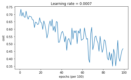
- Accuracy: 0.796666666667

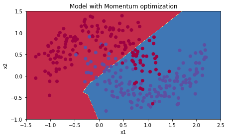
5.2 - Mini-batch gradient descent with momentum
# train 3-layer model
layers_dims = [train_X.shape[0], 5, 2, 1]
parameters = model(train_X, train_Y, layers_dims, beta = 0.9, optimizer = "momentum")

# Predict
predictions = predict(train_X, train_Y, parameters)

# Plot decision boundary
plt.title("Model with Momentum optimization")
axes = plt.gca()
axes.set_xlim([-1.5,2.5])
axes.set_ylim([-1,1.5])
plot_decision_boundary(lambda x: predict_dec(parameters, x.T), train_X, train_Y)
- Cost after epoch 0: 0.690741
- Cost after epoch 1000: 0.685341
- Cost after epoch 2000: 0.647145
- Cost after epoch 3000: 0.619594
- Cost after epoch 4000: 0.576665
- Cost after epoch 5000: 0.607324
- Cost after epoch 6000: 0.529476
- Cost after epoch 7000: 0.460936
- Cost after epoch 8000: 0.465780
- Cost after epoch 9000: 0.464740
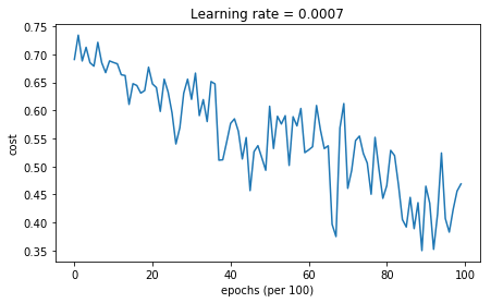
- Accuracy: 0.796666666667
5.3 - Mini-batch with Adam mode
# train 3-layer model
layers_dims = [train_X.shape[0], 5, 2, 1]
parameters = model(train_X, train_Y, layers_dims, optimizer = "adam")
# Predict
predictions = predict(train_X, train_Y, parameters)
# Plot decision boundary
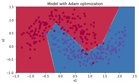
plt.title("Model with Adam optimization")
axes = plt.gca()
axes.set_xlim([-1.5,2.5])
axes.set_ylim([-1,1.5])
plot_decision_boundary(lambda x: predict_dec(parameters, x.T), train_X, train_Y)
- Cost after epoch 0: 0.690552
- Cost after epoch 1000: 0.185567
- Cost after epoch 2000: 0.150852
- Cost after epoch 3000: 0.074454
- Cost after epoch 4000: 0.125936
- Cost after epoch 5000: 0.104235
- Cost after epoch 6000: 0.100552
- Cost after epoch 7000: 0.031601
- Cost after epoch 8000: 0.111709
- Cost after epoch 9000: 0.197648
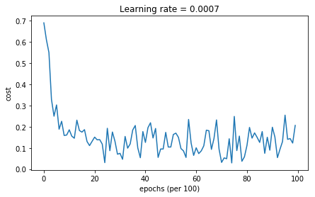
- Accuracy: 0.94
5.4 Summary
Momentum usually helps, but given the small learning rate and the simplistic dataset, its impact is almost negligeable. Also, the huge oscillations you see in the cost come from the fact that some minibatches are more difficult thans others for the optimization algorithm.
Adam on the other hand, clearly outperforms mini-batch gradient descent and Momentum. If you run the model for more epochs on this simple dataset, all three methods will lead to very good results. However, you’ve seen that Adam converges a lot faster.
Some advantages of Adam include:
- Relatively low memory requirements (though higher than gradient descent and gradient descent with momentum)
- Usually works well even with little tuning of hyperparameters (except α)